The Only 5 PromQL Queries You Really Need to Monitor a Linux Server

June 11, 2026

PromQL has its quirks, and can be difficult, but basic monitoring of a Linux server is not. I’ve boiled it down to five queries that will give you the basic outline of how your system is performing. This article discusses the queries for CPU, memory, disk space, disk IO, and network, with a plain explanation of how each one works.

PromQL has a reputation for being intimidating, and the reputation is half-earned. The full language is genuinely deep, with subtleties around ranges, rates, and vector matching that take a while to learn and understand. What nobody tells you when you are starting out is that monitoring a single Linux box well does not require a comprehensive grasp of the language. It requires about five questions, asked correctly.

// TL;DR

You don’t need hundreds of metrics to monitor a Linux server effectively. Five PromQL queries covering CPU, memory, disk space, disk IO, and network traffic will catch the most common server issues. This article explains each query, how it works, and why it belongs on your dashboard.

These queries work with both node_exporter and Grafana Alloy and are commonly used in Grafana dashboards, Prometheus alert rules, and Linux server monitoring setups. If you’re looking for practical PromQL examples rather than a full PromQL tutorial, start here.

// QUICK REFERENCE

These are the exact PromQL queries used to monitor CPU usage, memory utilization, disk space, disk IO, and network throughput on Linux servers running node_exporter or Grafana Alloy.

CPU Usage:    100 - (avg by (instance) (rate(node_cpu_seconds_total{mode="idle"}[5m])) * 100)
Memory Usage: 100 * (1 - (node_memory_MemAvailable_bytes / node_memory_MemTotal_bytes))
Disk Space:   100 - (node_filesystem_avail_bytes{fstype!~"tmpfs|overlay"} / node_filesystem_size_bytes{fstype!~"tmpfs|overlay"} * 100)
Disk IO:      rate(node_disk_io_time_seconds_total[5m])
Network:      rate(node_network_receive_bytes_total{device!~"lo|veth.*"}[5m])

This article assumes you have node_exporter or Grafana Alloy running and Prometheus scraping it. Alloy’s metrics are identical to node_exporter’s (Alloy’s prometheus.exporter.unix component is node_exporter under the hood), so every query below works for both. If you are still deciding between the two or would like to learn more, we wrote a separate comparison of Alloy and node_exporter that discusses the two and when each makes sense.

Before we dive into the queries, it’s important to point out the difference between a gauge and a counter on the Grafana dashboard. A gauge is a value that goes up and down, like memory in use right now or CPU temperature. It shows you what’s happening now, and you read a gauge directly. A counter only ever goes up, like total bytes received since boot or total seconds the CPU has spent working. It’s a count over time. You almost never read a counter directly, because “847 billion bytes since the machine booted” is useless. The relevant question to ask yourself when looking at counters is: how fast is it climbing? That’s what rate() tells you. Three of the five queries discussed below are counters, and once you see why they all use rate(), the pattern makes sense and PromQL starts to make a little more sense.

// 1. CPU USAGE (PERCENT BUSY)

100 - (avg by (instance) (rate(node_cpu_seconds_total{mode="idle"}[5m])) * 100)

When I created my first Grafana dashboard, I expected this to be the easiest query to write. I think most people expect it to be simple and, like me, are confused when it’s not.

node_exporter does not expose a “CPU percent” metric, because there is no honest single number for it. What it exposes is node_cpu_seconds_total, a counter that tracks how many seconds each CPU core has spent in each mode: idle, user, system, iowait, and a few others. The machine is always doing one of these, so the modes always add up to 100 percent of available CPU time.

The cleanest way to ask “how busy is the CPU” is to measure how much it is not idle, so we work from the idle mode and subtract from 100. Reading the query from the inside out:

• node_cpu_seconds_total{mode="idle"} selects just the idle counter, for every core.
• rate(...[5m]) is the key piece. It looks at how that counter changed over the last 5 minutes and returns a per-second rate. For the idle counter, the rate is “idle seconds accumulated per second,” which is a number between 0 and 1 per core: 1.0 means a core was fully idle, 0.0 means fully busy.
• avg by (instance) averages that across all the cores on the machine, so a 4-core box gives you one number instead of four.
• * 100 turns the 0-to-1 fraction into a percentage, and 100 - (...) flips “percent idle” into “percent busy.”

The [5m] window is a smoothing choice, not a magic number. A wider window like [5m] smooths out brief spikes and shows the server’s sustained load. If you use a narrower window like [1m] it’s twitchier and catches short bursts. For alerting on a server, sustained load is usually what matters, which is why our own default alert fires on CPU above 80 percent for five-plus minutes rather than reacting to every momentary peak. By extending the window from [1m] to [5m] you’re able to reduce noise, but can still see when there’s a problem.

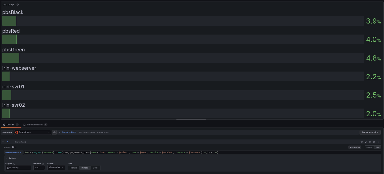
The production query adds label filters for multi-tenant use; the core logic is identical.

// 2. MEMORY USAGE (PERCENT USED)

100 * (1 - (node_memory_MemAvailable_bytes / node_memory_MemTotal_bytes))

Memory is best read as a gauge, so no rate() is used for this query. The values are read at a glance. There is one trap worth understanding, because it’s fairly common.

The naive instinct is to use node_memory_MemFree_bytes, the amount of completely unused memory. It’s a baseline metric that node_exporter provides, and it seems like it makes perfect sense to pull it directly to the panel. On a healthy Linux system, “free” memory is often very low by design. Linux uses otherwise-idle RAM for the page cache, holding recently-read files in memory so it does not have to hit the disk again. That memory looks “used” but is instantly reclaimable the moment a program actually needs it. If you track and alert on low MemFree, you’ll get unnecessary alerts on servers that are working as intended.

The number you need to track is node_memory_MemAvailable_bytes. The kernel calculates this for you. It is the memory genuinely available for new programs to use, after accounting for the cache it can reclaim.

So the query reads: take available memory divided by total memory, which gives you the fraction available. Subtract that from 1 to get the fraction used, and multiply by 100 for a percentage. A good threshold for this panel is 85 percent, or when available memory drops below 15 percent.

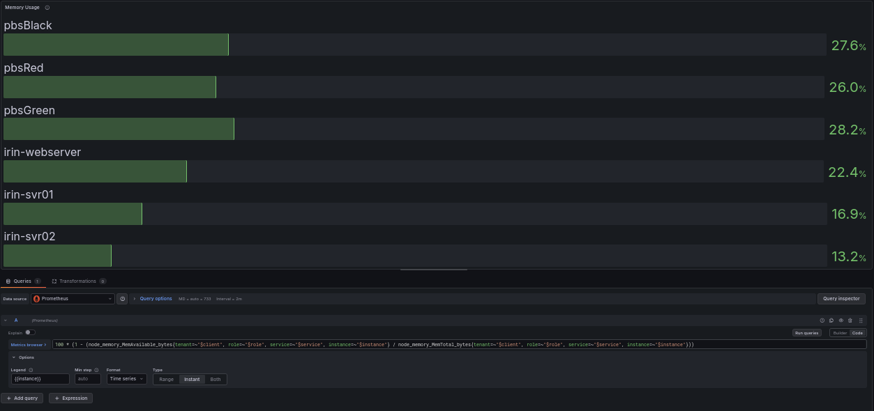
The production query adds label filters for multi-tenant use; the core logic is identical.

// 3. DISK SPACE (PERCENT FULL)

100 - (node_filesystem_avail_bytes{fstype!~"tmpfs|overlay"} / node_filesystem_size_bytes{fstype!~"tmpfs|overlay"} * 100)

Disk space is also a gauge, and structurally this is the same shape as the memory query. Take the available divided by total, and turn it into percent used. What makes this query tricky is the label filter, because disk monitoring using unfiltered queries can get noisy.

A Linux machine reports many “filesystems” that are not real disks. Tracking every single one would create a massive amount of noise, and make it difficult to parse out which disks are likely to cause a problem in the near future. tmpfs is memory-backed temporary storage, overlay filesystems belong to running containers, and there are others. If you monitor all of them, your “disk full” dashboard lights up over ephemeral mounts that are largely irrelevant. The filter fstype!~"tmpfs|overlay" strips those out:

• fstype is the label node_exporter attaches describing the filesystem type.
• !~ means “does not match this regular expression.” (=~ would be “does match.”)
• "tmpfs|overlay" is the regex: the | is an OR, so this matches either type, and !~ excludes both.

This query leaves you with the actual disks on your server. This is also the first time a regex-matching operator has appeared in this article. These two operators, =~ and !~, are how to do most of the flexible filtering in PromQL. Once you can include or exclude by pattern, you can filter metrics any way you need.

One caveat: this query returns one result per mounted disk, which will show metrics for each mounted drive on your server. A server with a separate / and /data should show you both, because either can fill independently. Setting the threshold to something like 85 percent full gives you time to act before the disk is full.

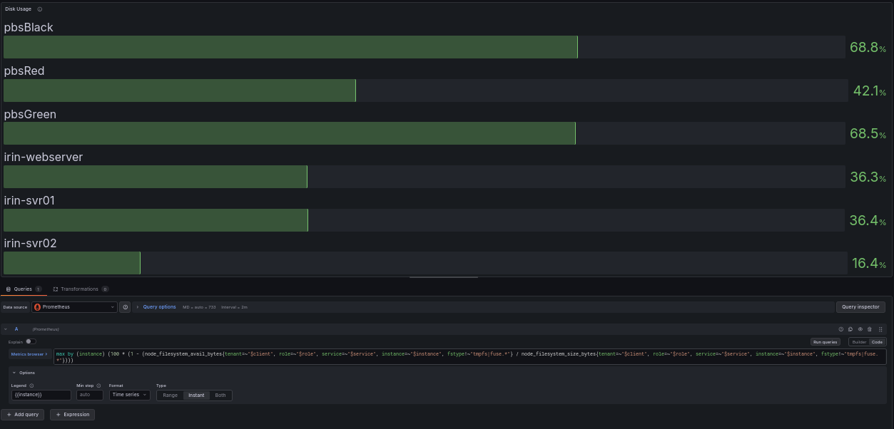
The production query adds label filters for multi-tenant use; the core logic is identical. The production query uses max by (instance) rather than the simplified version described above.

// 4. DISK IO (HOW SATURATED THE DISK IS)

rate(node_disk_io_time_seconds_total[5m])

The fourth query uses a counter, so rate() returns. This query answers a question that disk-space monitoring doesn’t address. Your disk can have plenty of free space and still create problems because it cannot read and write fast enough to keep up with what the system is demanding of it.

node_disk_io_time_seconds_total counts the total seconds the disk spent actively busy with input/output (IO). Because it is a counter, you wrap it in rate(...[5m]) to get “seconds of IO activity per second,” which is effectively a utilization fraction. A result near 1.0 means the disk was busy essentially the entire time, which tells you that the disk is saturated. A result near 0.1 means it was busy about 10 percent of the time, with plenty of headroom.

This is the metric that can help identify where slowdowns are coming from. When a database gets sluggish, or backups drag but CPU and memory look fine, disk IO saturation is very often the culprit. It’s the kind of problem that simple up-or-down monitoring won’t tell you.

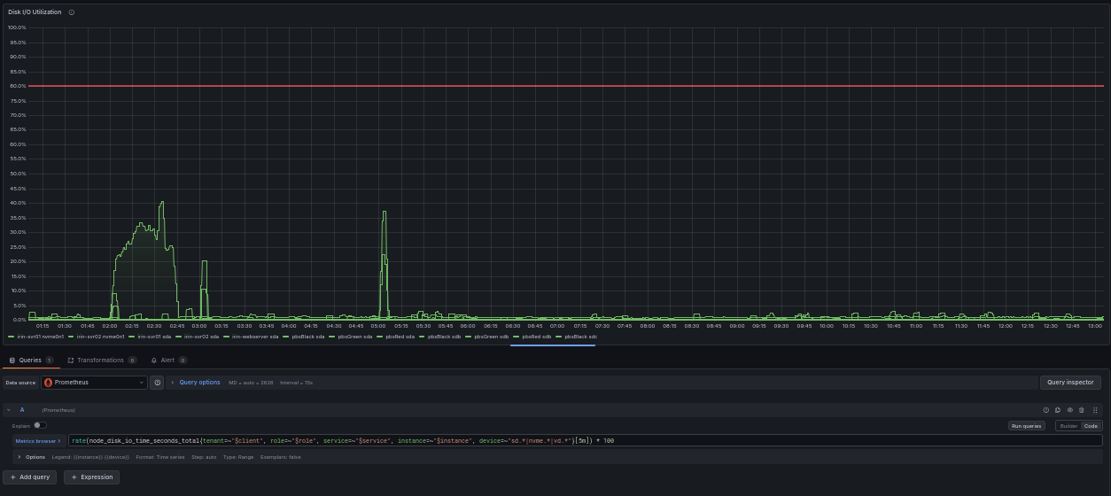
The production query adds label filters for multi-tenant use; the core logic is identical.

// 5. NETWORK THROUGHPUT (BYTES PER SECOND)

rate(node_network_receive_bytes_total{device!~"lo|veth.*"}[5m])

The fifth query is a counter and a regex filter together, which is why I saved it for last. If you understand this one fully, you’ll have a better understanding of the pattern behind all five.

node_network_receive_bytes_total is a counter of total bytes received on each network interface since boot. rate(...[5m]) turns it into bytes per second, your live inbound throughput. To watch outbound traffic, swap in node_network_transmit_bytes_total, or create a second query in your panel to view the two side by side.

The filter handles the same noise problem that the disk query does. A Linux host has interfaces that you typically don’t need to keep an eye on: lo is the loopback (the machine talking to itself), and veth interfaces are the virtual ethernet links Docker and other container runtimes create, often dozens of them. device!~"lo|veth.*" excludes them:

• lo matches the loopback exactly.
• veth.* is a regex where . means “any character” and * means “zero or more of the preceding,” so veth.* matches veth followed by anything: veth1a2b3c, vethABCD, all of them.

This leaves your physical or primary virtual interface(s), the one(s) carrying traffic that actually matters. The output is in bytes per second, so if you would rather see bits per second to compare against your network provider’s numbers, multiply by 8.

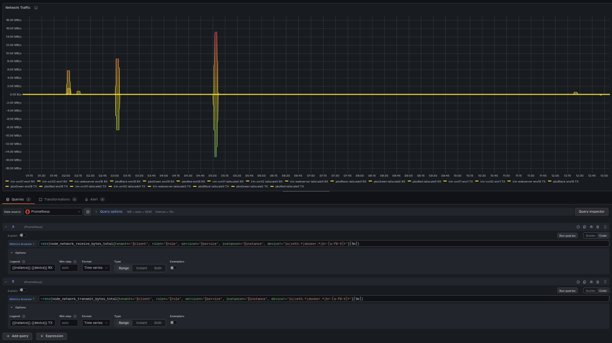
The production query adds label filters for multi-tenant use; the core logic is identical. TX is shown as negative so RX and TX can share one panel without overlap.

// THE PATTERN

Looking over the five queries discussed here, there are only a few moving parts. Gauges (memory, disk space) you read directly as available-over-total. Counters (CPU, disk IO, network) you wrap in rate() to ask how fast they are climbing. And label filters with =~ and !~ let you cut out the noise so you are watching real disks and real interfaces instead of container ephemera. Five queries, three ideas, and you have basic coverage of your servers.

// WHERE THIS LEAVES YOU

If you put these five on a dashboard with sensible thresholds, you have covered the large majority of what goes wrong on a single Linux server: the CPU is overworked, it runs out of memory, a disk fills up, a disk chokes, or its network saturates. There’s always more that you can monitor, and node_exporter and Alloy provide a massive amount of system metrics, but anything fancier is a refinement of these fundamentals. You can view Irin’s System Health dashboard here to see these five queries alongside a few others.

Going from “five queries in an expression browser” to “a real monitoring setup” is more work than it looks. Some of the gauge queries are modified and used as time series, so you can see what’s happening over time, not just in that instant. Prometheus needs to be set up to store the data with appropriate retention, Grafana dashboards need to be built around these queries, alert rules wired to thresholds that don’t create noise, and somewhere for the alerts to actually go. Setup isn’t overwhelming, but it is an ongoing process to keep it running and tuned. The monitoring system itself needs to be kept healthy, and thresholds and alerts need to be tuned to your system. Then there’s always the danger of over-monitoring: the first dashboard I created years ago was an endless scroll, it had everything, which turned out to be too much. Looking at the dashboard was overwhelming, and I couldn’t just take a glance at it to see how the system was doing, which is the goal.

That recurring chore is the gap Irin Observability exists to fill. We ship these exact queries, pre-built dashboards, and tuned alert thresholds (the 80-percent-CPU, 15-percent-memory, 85-percent-disk defaults referenced above are ours) as a flat-rate managed service, so you get the visibility without becoming the person who maintains the monitoring stack. But whether you run it yourself or hand it off, the five queries above are the foundation either way.

Once you’re familiar with these, the natural follow-up is wiring node_exporter or Alloy up properly and understanding what it can and cannot tell you on its own.